IF97 Steam/Water Properties

General Introduction

Steam/Water properties are of critical importance in industry and specifically the power industry. The standard for water properties is maintained by the International Association for the Properties of Water and Steam (IAPWS). The most recent formulation for thermodynamic properties is the Helmholtz formulation in IAPWS-95, which is exactly what the CoolProp HEOS backend uses when specifying the fluid as Water or HEOS::Water. The Helmholtz equations of state are based on \(T\) and \(\rho\) as state variables, so \(T, \rho\) will always be the fastest inputs, while \(p,T\) will be a bit slower (3-10 times). Inputs where neither \(T\) nor \(\rho\) are given, like \(P,H\), will be much slower.

Realizing the need for fast numerical computation of water properties, the IAPWS created a committee to develop a faster formulation for the steam power industry. In 1997, the IAPWS release the “IAPWS Industrial Formulation 1997 for the Thermodynamic Properties of Water and Steam” or IAPWS-IF97. This formulation replaced the older IFC-67 formulation. It is pressure based (rather than density based), and uses fundamental equations for the Gibbs free energy and its derivatives. While IAPWS-IF97 is faster, it is less accurate than the IAPWS-95 formulation, but within 1% uncertainty for all properties (and in many areas within 0.1%) except very near the critical point. Details of this formulation can be found in IAPWS-IF97, released in 2007 and updated in 2012.

The IF97 backend in CoolProp is based on the latest IAPWS Releases for thermodynamic and transport properties. It was originally coded as a fast water property calculation for the Humid Air backend. It has matured to include most of the forward and backward formulations in all fluid phase regions as released by the IAPWS and can provide a much faster calculation of water properties than the default HEOS backend (or the REFPROP backend, which is also based on IAPWS-95).

Piecewise structure of IAPWS-IF97

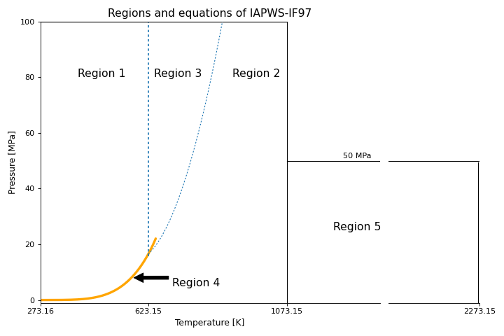
IAPWS-IF97 is piecewise by construction. The \((T, p)\) plane is partitioned into five regions, each with its own fundamental equation:

• Region 1 — compressed liquid (\(T \le 623.15\) K, below the saturation curve and above the melting curve). Backward Gibbs free energy \(g_1(T, p)\).

• Region 2 — superheated steam and high-\(T\) gas, from the saturation curve up to \(T = 1073.15\) K. Backward Gibbs \(g_2(T, p)\).

• Region 3 — dense supercritical and near-critical (\(T \ge 623.15\) K, \(p \ge p_{B23}(T)\)). Helmholtz \(f_3(\rho, T)\) in \((\rho, T)\) rather than \((p, T)\) — the only IF97 region not parameterised in pressure.

• Region 4 — saturation curve, \(p_\mathrm{sat}(T)\) only.

• Region 5 — high-temperature extension \(T \in [1073.15, 2273.15]\) K up to 50 MPa. Backward Gibbs \(g_5(T, p)\).

The boundaries between regions are themselves analytic curves:

• The R2/R3 boundary is the parametric curve \(p_{B23}(T) = 1.0193 \times 10^{-3} \cdot (T - 572.545)^2 + 13.919\) MPa, valid for \(T \in [623.15, 863.15]\) K (equivalently \(p \in [16.529, 100]\) MPa).

• The R1/R3 boundary is the isotherm \(T = 623.15\) K.

Because IF97 uses different fundamental equations across these curves, calorimetric and acoustic quantities (\(c_p, s, w\)) have structural kinks at the boundaries — the absolute values match across the boundary by construction, but derivatives do not. Any downstream interpolator built on IF97 (the SVDSBTL backend, in particular) must respect this structure to recover G13-15-conformant accuracy. A bilinear or bicubic table over a region that straddles \(p_{B23}\) averages the kink into the interpolant, producing percent-class structural error in \(v, s, w\) near the boundary (the SVDSBTL atlas split along \(p_{B23}\) was introduced specifically to avoid this regime). The right fix is to split the region along the kink and table each side independently.

A plot of the region atlas (orange = saturation curve, dashed = \(p_{B23}\) and \(T = 1073.15\) K boundaries) appears under Range of validity below.

IF97 Backend

The IF97 backend can be accessed the same way as the other backends, by prefixing the fluid name in calls to PropsSI and Props1SI. Water is the only fluid that can be specified, as IF97::Water (the alias IF97::H2O is also accepted, case-insensitively). Most output variables and input pairs are accepted as of CoolProp 6.1.1, with a few exceptions:

1. Generic Partial Derivatives are not yet supported.

2. Mixtures are obviously not supported since this is a Water-only backend.

3. Setting the reference state has no effect on IF97 properties (top-level set_reference_state(...) silently returns; the OO AbstractState::set_reference_stateS raises NotImplementedError). The reference state is fixed such that the specific internal energy, \(U\) , and the specific entropy, \(S\) , of the saturated liquid at the triple point are identically zero.

4. Solid properties are not supported in any of the ICE regions.

5. The melting-sublimation curve is not used; rather, the property equations are limited uniformly at \(T_{min}=273.15K\).

IF97 Range of Validity

Although IF97 is generally faster than the other backends, it is only applicable over a much smaller range of temperatures and pressures than the HEOS or REFPROP Water formulations. The IF97 properties are divided into several regions. The valid range of these regions is shown in the following plot. Attempts to retrieve properties outside of these regions will result in an “Out of Range” error.

(Source code, png, .pdf)

IF97 Water Property Examples

A call to the top-level function PropsSI can provide: temperature, pressure, density, specific heat, internal energy, enthalpy, entropy, speed of sound, viscosity, thermal conductivity, surface tension, and Prandtl Number. Hence, the available output keys are: T, P, D, C, Cvmass, U, H, S, A, V, L, I, and Prandtl. Molar quantities can also be returned, but IF97 is mass based. Trivial outputs, such as M, Tmin, Tmax, Pmin, Pmax, Ttriple, Tcrit, ptriple, and pcrit, are also available.

In [1]: from CoolProp.CoolProp import PropsSI

#Specific heat capacity of Water at 500 K and 1 atm
In [2]: PropsSI('C','T',500,'P',101325,'IF97::Water')
Out[2]: 1981.5422965970472

#Density of Water at 500 K and 1 atm.
In [3]: PropsSI('D','T',500,'P',101325,'IF97::Water')
Out[3]: 0.4409206435977277

#Round trip in thermodynamic properties
In [4]: T_init = 500.0

In [5]: P_init = 101325

In [6]: S_init = PropsSI('S','T',T_init,'P',P_init,'IF97::Water')

In [7]: H_init = PropsSI('H','S',S_init,'P',P_init,'IF97::Water')

In [8]: T_final = PropsSI('T','H',H_init,'P',P_init,'IF97::Water')

#Round trip complete.  T_final should match T_init
In [9]: T_final
Out[9]: 499.99805290471727

#Saturation pressure of Water at 500 K (Q can be 0 or 1)
In [10]: PropsSI('P','T',500,'Q',0,'IF97::Water')
Out[10]: 2638897.7562732203

#Saturated LIQUID enthalpy of Water at 500 K (Q = 0)
In [11]: H_L = PropsSI('H','T',500,'Q',0,'IF97::Water'); print(H_L)
975464.7957611234

#Saturated VAPOR enthalpy of Water at 500 K (Q = 1)
In [12]: H_V = PropsSI('H','T',500,'Q',1,'IF97::Water'); print(H_V)
2802589.9096435737

#Latent heat of vaporization of Water at 500 K
In [13]: H_V - H_L
Out[13]: 1827125.1138824504

#Critical temperature for Water
In [14]: PropsSI('Tcrit','T',0,'P',0,'IF97::Water')
Out[14]: 647.096

#Triple Point pressure for Water
In [15]: PropsSI('ptriple','T',0,'P',0,'IF97::Water')
Out[15]: 611.657

IF97 Conformance and Timing

Note

All tables and figures in this section are regenerated by Web/scripts/fluid_properties.IF97Conformance.py on every docs build, against the local CoolProp commit. The numbers shipped with the published docs come from the GitHub-hosted CI runner; rebuild locally to see numbers for your hardware and source revision.

Conformance is measured against the IAPWS G13-15 Tables 8-13 (Kunick et al., 2015) protocol: for each IF97 region we draw 50000 random \((p, T)\) samples log-uniform in \(p\) and uniform in \(T\), classify them into the IF97 region atlas, compute \(h = h_\mathrm{IF97}(p, T)\), evaluate each tested backend at \((h, p)\), and tabulate the maximum and root-mean-square deviation from IAPWS-IF97 of the six properties in G13-15: \(T(p,h)\), \(v(p,h)\), \(s(p,h)\), \(w(p,h)\), \(\eta(p,h)\), \(\lambda(p,h)\). Region 4 (saturation dome) is excluded — G13-15 evaluates the forward / backward equations only outside the dome.

Deviation of SVDSBTL&IF97::Water from IAPWS-IF97

The figure below shows where the failures live in \((p, h)\) coords across the full IF97 envelope — six panels, one per G13-15 property (\(T, v, s, w, \eta, \lambda\)). Only the budget-violating probes are plotted; marker size and colour both encode \(\log_{10}(|\Delta| / |\Delta|_\mathrm{perm})\), so bigger + redder is further past budget. Overlays: the saturation dome, the IF97 R1/R3 isotherm (\(T = 623.15\) K) and R2/R5 isotherm (\(T = 1073.15\) K), the R2/R3 boundary curve \(p_{B23}(T)\), and the auto-calibrated critical-patch HEOS-fallback bbox (gold). Black dot marks the critical point.

The clustering pattern is the load-bearing signal — it tells you why the table fails where it does, and what to do about it:

• Thermodynamic panels (\(T, v, s, w\)): failures cluster around the critical point (rank-20 SVD cannot represent the \((\partial \rho / \partial p)_h\) cusp at the critical singularity — that would require unbounded rank). The gold critical-patch bbox covers the bulk of those failures; the auto-calibration loop sized it to do exactly that. Residual reds outside the gold bbox are thin-Hermite-support corner cells (CoolProp-3c4 accuracy ceiling — accepted, not fixable by widening the bbox).

• Transport panels (\(\eta, \lambda\)): failures are widespread. The G13-15 transport budgets (\(10^{-5}\) relative) are 100-1000x tighter than the thermodynamic ones, and the rank-20 SVD’s representation of viscosity / conductivity is not yet conformant — closing this gap is tracked in the SBTL conformance epic (CoolProp-foi). The thermodynamic panels are the ones to focus on when assessing whether SVDSBTL is fit-for-purpose for a given application; the transport panels document the remaining work.

• The R2/R3 kink along \(p_{B23}(T)\) is no longer a structural failure cluster — the atlas split introduced in CoolProp-foi.9.5 separates SUPER_R2 and SUPER_R3 so each SVD only sees cells on one side of the kink. Residual failures along that line are the boundary-row cells where the Hermite kernel spans across \(p_{B23}\).

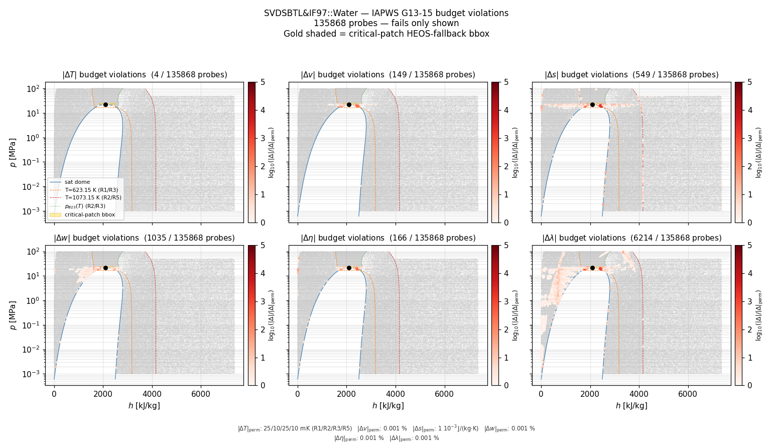
SVDSBTL&IF97::Water — IAPWS G13-15 budget violations across the full IF97 envelope.

Download the same figure as a vector PDF (~14 MB; useful for print / slides).

G13-15 Table 8 — \(T(p,h)\), permissible \(|\Delta T|_\mathrm{perm}\) is region-dependent (per-region column below).

IF97 Region	in-region samples	\(|\Delta T|_{\mathrm{perm}}\) \([\mathrm{mK}]\)	\(|\Delta T|_{\max}\) \([\mathrm{mK}]\)	\((\Delta T)_{\mathrm{RMS}}\) \([\mathrm{mK}]\)
1	23339	25	2.79	0.0589
2	38532	10	8.52	0.0968
3	23333	25	192	1.48
5	50000	10	1.84	0.0247

G13-15 Table 9 — \(v(p,h)\), permissible \(|\Delta v|_\mathrm{perm} = 0.001\ \%\).

IF97 Region	in-region samples	\(|\Delta v|_{\max}\) \([\%]\)	\((\Delta v)_{\mathrm{RMS}}\) \([\%]\)
1	23339	0.00378	5.24e-05
2	38532	0.00342	3.23e-05
3	23333	1.24	0.00867
5	50000	0.000766	1.1e-05

G13-15 Table 10 — \(s(p,h)\), permissible \(|\Delta s|_\mathrm{perm} = 1\ 10^{-3}\ \mathrm{J/(kg\,K)}\).

IF97 Region	in-region samples	\(|\Delta s|_{\max}\) \([10^{-3}\ \mathrm{J/(kg\,K)}]\)	\((\Delta s)_{\mathrm{RMS}}\) \([10^{-3}\ \mathrm{J/(kg\,K)}]\)
1	23339	29.2	0.43
2	38532	38.5	0.374
3	23333	9.44e+03	64.5
5	50000	13.2	0.182

G13-15 Table 11 — \(w(p,h)\), permissible \(|\Delta w|_\mathrm{perm} = 0.001\ \%\).

IF97 Region	in-region samples	\(|\Delta w|_{\max}\) \([\%]\)	\((\Delta w)_{\mathrm{RMS}}\) \([\%]\)
1	23339	0.036	0.000627
2	38532	0.00442	4.87e-05
3	23333	0.283	0.00334
5	50000	0.000259	3.62e-06

G13-15 Table 12 — \(\eta(p,h)\), permissible \(|\Delta \eta|_\mathrm{perm} = 0.001\ \%\).

IF97 Region	in-region samples	\(|\Delta \eta|_{\max}\) \([\%]\)	\((\Delta \eta)_{\mathrm{RMS}}\) \([\%]\)
1	23339	0.0346	0.000374
2	38532	0.0038	4.93e-05
3	23333	1.2	0.00837
5	50000	0.000907	1.15e-05

G13-15 Table 13 — \(\lambda(p,h)\), permissible \(|\Delta \lambda|_\mathrm{perm} = 0.001\ \%\).

IF97 Region	in-region samples	\(|\Delta \lambda|_{\max}\) \([\%]\)	\((\Delta \lambda)_{\mathrm{RMS}}\) \([\%]\)
1	23339	0.0321	0.00232
2	38532	0.0366	0.0005
3	23333	6.3	0.0439
5	50000	0.00112	1.49e-05

Backend timing (AbstractState.update regime)

Two tables below time the same backends against the same sample population for both PT_INPUTS (the input pair the conformance sweep is drawn on) and HmassP_INPUTS (the input pair most users actually call with — the whole point of a tabulated backend is the cheap \((h, p)\) lookup). Sample points are identical across the two tables; only the input pair changes. \(h(T, p)\) is taken from the reference IF97 backend so HmassP inputs are forward-consistent with PT inputs.

Each cell is the mean wall time for one ``update()`` + one ``keyed_output()`` requesting that property — i.e. one output per call. Backends that share the flash across N outputs would amortise this measurement; the SVDSBTL fast_evaluate path is the batched variant. The ratio column is the mean across the per-property ratios \(t_{\mathrm{backend}} / t_{\mathrm{IF97}}\) for that input pair. Lower is faster than IF97. Rows are sorted by descending mean ratio so the slowest path sits at the top. Absolute timings depend on hardware; the ratios are the load-bearing quantity. CI rebuilds these on a GitHub-hosted runner.

PT_INPUTS:

Backend	T	D	A	V	mean ratio vs IF97
IF97::Water	145 ns	524 ns	1.54 us	617 ns	1.00
SVDSBTL&IF97::Water	234 ns	426 ns	423 ns	454 ns	0.86

HmassP_INPUTS:

Backend	T	D	A	V	mean ratio vs IF97
IF97::Water	11.72 us	12.41 us	14.28 us	12.29 us	1.00
SVDSBTL&IF97::Water	543 ns	548 ns	549 ns	570 ns	0.04

SVDSBTL&IF97 — open-source, fast, fully traceable

The conformance section above tests one configuration: SVDSBTL&IF97::Water, where SVDSBTL serves as a tabulated interpolator over the IAPWS-IF97 source equations. Why is this useful when the SBTL backend (an existing CoolProp tabular backend based on cubic B-splines) already exists?

• Open source. SVDSBTL is built on the SVD components shipped with CoolProp itself (see Low-rank SVD lookup for 2D property tables). No proprietary closed-source dependencies, no licensed binaries — everything that goes into building the tables ships in the source tree. Anyone can reproduce the bit-identical table by re-running the build with the same source revision.

• High speed. The three performance regimes cover the full single-shot-to-CFD-scale range. The per-output marginal cost in the batched fast_evaluate path is ~35 ns on Apple Silicon (supercritical region; mixes that touch the critical patch heavily can rise to ~1 µs/probe) — competitive with the fastest closed tabular implementations.

• Complete traceability. Every cell of the table is reproducible from the source backend at the exact build-time source revision. The cache file stores the options hash that generated it, so two installs sharing the same fluid + source + options recompute bit-identical tables; mismatches force a rebuild instead of silently mixing revisions. This matters whenever the table is part of a regulated calculation chain (industrial control, certification, scientific publication).

These three properties together set SVDSBTL apart from the older SBTL backend and from closed-source tabulators. The conformance figures above characterise how the four G13-15 thermodynamic properties (\(T, v, s, w\)) fare against per-region IAPWS budgets — see the SVDSBTL accuracy envelope section for the per-property/per-region pass/fail summary.

IF97 vs HEOS timing — per-call and batched

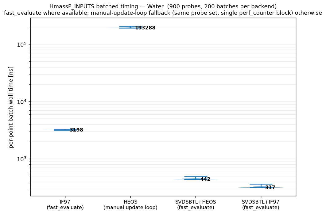
The figure below profiles AbstractState.update(HmassP_INPUTS, h, p) for every backend the local build exposes (IF97, HEOS, and the SVDSBTL family when bound through Python). It also reports CoolProp.AbstractState.fast_evaluate() — a cache-bypassing zero-allocation batch path — for backends that implement it (currently IF97 and the tabular backends). The profile script regenerates the figure against your local hardware and CoolProp build; the numbers shipped with the docs come from the GitHub-hosted CI runner.

Per-call panels report the median wall time over many warm-cache calls (first-call cache-load cost is baked out). Per-call numbers include ~300 ns of Cython-wrapper marshalling across the three FFI crossings (update + two accessors) that applies equally to every backend — read the ratios as the meaningful comparison, not the absolute nanoseconds. fast_evaluate amortizes that overhead over the batch, so its per-point cost approaches the native floor — sub-µs for the tabular backends (SVDSBTL ~300 ns/probe in the supercritical region), while bare IF97’s own \((p, h)\) inversion stays ~2 µs/probe regardless of the wrapper. IF97’s own dome-blend lever-rule path was added in CoolProp 7.2.1 (PR #2942), so probes landing inside the saturation dome no longer return NaN through fast_evaluate — they Q-blend between IF97’s saturation endpoints.