SVDSBTL — SVD-Compressed Tabular Lookup Backend

SVDSBTL is a tabular-lookup backend that combines an atlas of analytically-bounded regions with a low-rank SVD of each region’s property surfaces. It produces sub-microsecond property evaluations in the batched fast_evaluate path away from the critical patch (~300-400 ns per probe at four outputs on Apple Silicon, rising to a few µs/probe inside the critical-patch fallback), at IAPWS G13-15 \(T(p, h)\) conformance for water and a single-digit percent accuracy ceiling for the multi-fluid HEOS-backed presets, at a disk footprint of ~7-14 MB per (fluid, input pair, source backend).

This page is the user-facing page: how to use the backend, what it guarantees, and when to pick it. For the underlying SVD math (rank-\(r\) reconstruction, cubic Hermite slopes, axis transforms), see Low-rank SVD lookup for 2D property tables.

What it is

A traditional bicubic table covers the full \((p, h)\) or \((p, T)\) envelope with one coarse grid and stores the source backend’s property values at each cell. Two known limitations of that approach: (a) the saturation boundary can’t be expressed on a regular grid without padding cells on either side, so a single table either crosses the dome (with the discontinuity smearing into the bicubic interpolant) or excludes a stripe around it (so the backend can’t answer there); and (b) memory grows quadratically with grid resolution — the bicubic table for a single fluid at useful accuracy is hundreds of MB. SVDSBTL replaces the single bicubic table with three layered components that address both:

1. Region atlas. The thermodynamic envelope is partitioned into ~3-7 disjoint regions in \((p, h)\) or \((p, T)\) — LIQUID (subcooled), VAPOR (superheated), SUPER (supercritical), with further splits for IF97 (R1/R3, R2/R3 boundary curves). Each region’s secondary axis is normalised to \([0, 1]\) via two analytic boundary curves — on subcritical regions one curve is the saturation dome and the other is an EOS-domain floor/ceiling (for the liquid region the floor walks up over the melting curve where it binds at high p, falling back to the low-T EOS isotherm where it doesn’t; for the vapor region the ceiling is the high-T isotherm at the EOS validity limit); on supercritical regions both curves are isotherms. Lookups first AABB-test against region bounding boxes (cheap), then evaluate the precise boundary curves on the candidate.

2. Per-region SVD. Inside each normalised region, every tabulated property (\(\rho, h, s, u, w, \eta, \lambda\)) is represented as a rank-\(r\) SVD of a dense \(N_h \times N_p\) (default \(200 \times 800\), \(r = 20\)) sample grid — the 200-point axis is the secondary (h or T), the 800-point axis is the primary (log p). Per-mode tensor-product cubic Hermite (1D × 1D, summed across rank-\(r\) modes) gives \(C^1\) continuity at minimum, and \(C^2\) with the default natural-cubic-spline slope source (see Low-rank SVD lookup for 2D property tables). Density and transport properties use a log transform (\(\rho = \exp(\sum_k S_k U_k V_k)\)) so their multi-decade dynamic range fits the SVD’s smoothness assumption.

3. Critical-patch HEOS fallback. Near the critical point the rank-truncated SVD cannot resolve the cusp in \((\partial \rho / \partial p)_h\) — a single dense region needs unbounded rank. SVDSBTL identifies a small rectangular patch in \((T, p)\) around the critical point (auto-calibrated per fluid; see Critical-patch bbox below) and routes queries inside the patch directly through the source backend. Outside the patch the SVD owns the answer; this keeps the SVD’s per-cell rank low everywhere else.

Queries through the public AbstractState interface dispatch to whichever of these three handles the input pair: the atlas locates the region, the per-region SVD returns the property, and the patch overrides when the query is in the critical neighbourhood. Two-phase dome queries lever-rule-blend between the source backend’s saturation endpoints (or Superancillaries when the source exposes one).

Constructor & supported pairs

SVDSBTL is constructed via the factory string SVDSBTL&<source>, where <source> is the truth-source backend that the SVD samples from at table-build time:

import CoolProp.CoolProp as CP

AS = CP.AbstractState("SVDSBTL&IF97", "Water")     # IAPWS G13-15
AS = CP.AbstractState("SVDSBTL&HEOS", "Methane")   # multi-fluid HEOS
AS = CP.AbstractState("SVDSBTL&REFPROP", "Water")  # REFPROP truth

The currently-supported source backends are HEOS, REFPROP, and IF97 (water only). SVDSBTL without a source backend (SVDSBTL alone) is intentionally not supported — there is no default truth source, since the choice changes both the sampled property values and the cache filename.

Two input pairs are currently tabulated per fluid:

• HmassP_INPUTS (the dominant industrial use case)

• PT_INPUTS (where the user already has \((p, T)\) and wants to skip the inverse \(T(p, h)\) solve)

HmolarP_INPUTS is served from the HmassP_INPUTS table by multiplying by molar mass. Two-phase PQ_INPUTS and QT_INPUTS route directly through the source’s saturation line — no separate table is required.

A planned follow-up adds HmassSmass and Dmass-Umass for the remaining G13-15 input-pair coverage (Tables 14-17); see bd CoolProp-phv.

The on-disk table cache

The first construction for a given (fluid, source, input_pair, options) tuple samples ~160,000 \((p, h)\) or \((p, T)\) points per region from the source backend (3 regions for HEOS-PH, 6-7 for IF97-PH, so 0.5-1.1M samples per table), runs SVD on each region’s property matrix, and persists the result as a zlib- compressed binary file under

$HOME/.CoolProp/SVDTables/<Fluid>.<Source>.<InputPair>.<OptHash>.svd.bin.z

(or under ${ALTERNATIVE_SVDTABLES_DIRECTORY}/ in place of $HOME/.CoolProp/SVDTables/ when that config key is set — see Configuration keys below). Subsequent constructions for the same tuple load from this cache.

• Build time: ~10-60 s per (fluid, input pair) on a 2024-era laptop, HEOS-source. REFPROP-source is several times slower (REFPROP flash per sample point).

• Disk footprint: ~5-15 MB per file depending on region count.

• Cache invalidation: the on-wire revision is checked on load. Changes to the serializer format, sampling code, or preset geometry bump the revision and force a rebuild. Source-code paths that affect the cached output are hashed into the GHA cache key in .github/workflows/test_catch2.yml so CI rebuilds occur automatically.

The cache directory defaults to ~/.CoolProp/SVDTables/ on all platforms. The location is configurable via the ALTERNATIVE_SVDTABLES_DIRECTORY configuration key — see Configuration keys below.

Three performance regimes

SVDSBTL exposes three distinct call patterns with very different per-call cost. Picking the right one matters far more than picking the backend.

1. AbstractState.update — reuse the instance (canonical path). Construct the AbstractState once, then call update / property accessors in a loop. Table load is amortised over the full workload:

   In [1]: import CoolProp.CoolProp as CP
   
   In [2]: from CoolProp import AbstractState
   
   In [3]: import numpy as np
   
   In [4]: AS = AbstractState("SVDSBTL&IF97", "Water")
   
   In [5]: h_arr = np.linspace(2.0e5, 3.0e6, 5)
   
   In [6]: p_arr = np.full_like(h_arr, 1.0e6)
   
   In [7]: def loop():
      ...:     for h, p in zip(h_arr, p_arr):
      ...:         AS.update(CP.HmassP_INPUTS, h, p)
      ...:         AS.rhomass(); AS.T()
      ...: 
   
   In [8]: %timeit loop()
   3.49 us +- 4.77 ns per loop (mean +- std. dev. of 7 runs, 100,000 loops each)
   

   Native C++ update + rhomass + T is region-dependent: well under 200 ns/call in single-phase (subcooled liquid, superheated vapor, supercritical), and ~1-1.5 µs/call in two-phase / sat-line regions where the SuperAncillary or source-backend PQ flash runs per probe. The cached accessors are <10 ns/pair on top. The Cython wrapper adds ~0.3 µs across the three FFI crossings — so even a Python loop sweeping the saturation dome stays ~20× faster than the same loop on HEOS. This path is fine for ad-hoc / setup code; for throughput-sensitive workloads, prefer fast_evaluate (next regime) which strips the per-probe wrapper marshalling and amortises locate + basis setup across multiple outputs.

2. fast_evaluate (batched, no instance mutation). AbstractState.fast_evaluate(input_pair, val1[], val2[], outputs[], out_buffer, status) writes N property values for M probes directly into a caller-supplied buffer. No per-point AbstractState cache mutation, no Python wrapper marshalling per probe, and shared \((p, h)\) locate / Hermite-basis setup across the N requested properties:

   The probe distribution below is supercritical only (\(p > p_c\), \(h > h_c\)) — this isolates the representative locate + basis cost from the critical patch, which is several µs/probe and would otherwise dominate a uniformly sampled \((p, h)\) box:

   In [9]: import CoolProp.CoolProp as CP
   
   In [10]: from CoolProp import AbstractState
   
   In [11]: import numpy as np
   
   In [12]: AS = AbstractState("SVDSBTL&IF97", "Water")
   
   In [13]: N = 10_000
   
   In [14]: rng = np.random.default_rng(0)
   
   In [15]: h = rng.uniform(2.5e6, 4.0e6, N)   # h > h_c ≈ 2086 kJ/kg
   
   In [16]: p = rng.uniform(22.5e6, 50.0e6, N) # p > p_c = 22.064 MPa
   
   In [17]: outputs = np.array([CP.iT, CP.iDmass, CP.iSmass, CP.iUmass], dtype=np.int32)
   
   In [18]: out = np.empty((N, 4)); status = np.empty(N, dtype=np.int32)
   
   In [19]: %timeit AS.fast_evaluate(CP.HmassP_INPUTS, h, p, outputs, out, status)
   5.14 ms +- 2.93 us per loop (mean +- std. dev. of 7 runs, 100 loops each)
   

   Per-point wall time: ~300-330 ns for a 4-output query on Apple Silicon (10k-probe batch, supercritical region). Marginal cost per added surface output is ~35 ns from a linear fit over \(N_{\mathrm{out}} \in \{1, \dots, 5\}\) — setup intercept ~170 ns covers the per-probe locate + basis-weight evaluation that is shared across the requested outputs. For CFD-scale workloads (≥100k probes per timestep) this is the only sensible API. Uniformly-sampled \((p, h)\) boxes that touch the critical patch heavily can rise to ~1 µs/probe; pure supercritical or PT sweeps hold the headline number.

3. PropsSI — the high-level wrapper (off by default). PropsSI is the high-level entry point that resolves the backend and constructs an AbstractState on every call. For SVDSBTL that means a zlib-decompressed .svd.bin.z load (~80 ms for the typical ~7 MB table, ~140 ms for the larger 14 MB SVDSBTL&IF97 HmassP table). For a one-off interactive query this is fine; for a throughput workload it is catastrophic — every PropsSI call pays the table-load cost again.

   SVDSBTL therefore opts out of PropsSI by default. Enable only for interactive / scripting use where the construction cost is irrelevant:

   CP.set_config_bool(CP.ALLOW_SVDSBTL_IN_PROPSSI, True)
   CP.PropsSI("D", "T", 500.0, "P", 1e6, "SVDSBTL&IF97::Water")
   

   This gate is enforced architecturally — the same pattern the bicubic and TTSE backends use, for the same reason.

The profile figure on the IF97 page shows all three regimes side-by-side, against HEOS and IF97 baselines.

Critical-patch bbox

Near the critical point the rank-\(r\) SVD’s reconstruction error diverges — the \((\partial \rho / \partial p)_h\) cusp at the critical singularity needs unbounded rank to represent, and even a generous rank like \(r = 20\) leaves multi-percent error in \(\rho\) and ten-percent-class error in \(w\) within a fraction of \(T_c\) from the critical point. SVDSBTL covers this slice with a small axis-aligned rectangular patch in \((T, p)\): every query whose state lands inside the patch forwards to the source backend (HEOS / REFPROP / IF97) for the calculation; everything outside the patch goes through the SVD.

Patch shape per fluid. The patch is computed automatically at the first backend construction for a given (fluid, source backend, options) combination, via a binary-search shrink loop:

1. Start from the Water-sized default \([0.95, 1.05] T_c \times [0.75, 1.15] p_c\).

2. For each of the four axes \((T_\mathrm{lo}, T_\mathrm{hi}, p_\mathrm{lo}, p_\mathrm{hi})\), binary-search-shrink the multiplier toward 1.0 (= the critical point) until the SVD’s reconstruction at a strip of probes just outside the candidate patch boundary passes the calibration error budget against the source backend (1% relative in \(\rho, h, s\); 5% relative in \(w\)).

3. The result is persisted to a sidecar file alongside the .svd.bin.z table caches:

   $HOME/.CoolProp/SVDTables/<Fluid>.<Source>.critpatch.<OptHash>.bin
   

   Subsequent constructions load the cached multipliers; the calibration probe is not re-run.

The calibrator never widens the patch beyond the Water default — so Water keeps its tested bbox and other fluids tighten only as much as their critical-singularity footprint allows. Typical results (post-CoolProp-5ni / -dxd):

Fluid (source)	\(T_\mathrm{lo} / T_c\)	\(T_\mathrm{hi} / T_c\)	\(p_\mathrm{lo} / p_c\)	\(p_\mathrm{hi} / p_c\)
Water (HEOS)	0.986	1.025	0.996	1.150
Water (IF97)	0.999	1.010	0.996	1.138
CarbonDioxide (HEOS)	0.994	1.050	0.996	1.150
R134a (HEOS)	0.999	1.001	0.996	1.014

These numbers are regenerated at backend construction; the exact values are sensitive to the SVD grid size and rank (and so move when the options blob changes). CoolProp-3c4 tracks the residual accuracy ceiling at extreme thin-support cells outside the patch, which the calibrator deliberately ignores (axis-aligned bboxes can’t cover those scattered failures).

For the HmassP_INPUTS input pair the \((p, h)\) bbox is derived from the \((T, p)\) patch by walking the perimeter through the source backend’s \(h(T, p)\) and taking the axis-aligned envelope of the resulting \(h\) values — that way any \((T, p)\) in the canonical patch round-trips into a \((h, p)\) that the patch test also fires on. For Water/HEOS the resulting \((p, h)\) bbox is roughly \(p \in [22.0, 25.4]\) MPa, \(h \in [1.74, 2.65]\) MJ/kg.

Overrides. Two escape hatches:

• critical_patch.bbox in the options JSON — set explicit \((T_\mathrm{lo}, T_\mathrm{hi}, p_\mathrm{lo}, p_\mathrm{hi})\) multipliers (skips auto-calibration entirely). Useful for pinning the patch to a known-good shape across versions.

• critical_patch.mode = "off" — disables the patch. Queries near the critical point will return the SVD’s rank-truncated reconstruction with the corresponding accuracy degradation. Useful for benchmark studies of the SVD itself.

• critical_patch.mode = "fixed" — enables the patch but skips the auto-calibration shrink loop. The patch uses whatever critical_patch.bbox the caller supplied; if bbox is omitted, the Water-sized default \([0.95, 1.05] T_c \times [0.75, 1.15] p_c\) is used as-is. Useful when you want to lock the patch geometry to a known shape across CoolProp versions without paying the per-fluid calibration cost.

• critical_patch.source — override the source backend that serves in-patch queries. E.g. SVDSBTL&IF97 with critical_patch.source = "HEOS" uses IF97 for the SVD truth source but HEOS for in-patch queries (which gives full IAPWS-95 accuracy at the critical singularity rather than IF97’s R3 formulation).

Configuration keys

ALLOW_SVDSBTL_IN_PROPSSI (default false)

Gate for PropsSI routing. See Three performance regimes. Set to true for interactive use; leave false for throughput code.

ALTERNATIVE_SVDTABLES_DIRECTORY (default empty)

Override the on-disk cache directory. When non-empty, both the .svd.bin.z surface files and the .critpatch.bin sidecars are read from and written to this directory in place of the default ~/.CoolProp/SVDTables/. The directory is created on first use. Useful when $HOME is read-only (CI containers, sandboxed processes), on shared workstations, or when a centrally-managed cache is preferable. Set via the Python API like any other string-typed config key:

import CoolProp.CoolProp as CP
CP.set_config_string(CP.ALTERNATIVE_SVDTABLES_DIRECTORY, "/srv/coolprop_cache")

SVDSBTL_SAMPLING_THREADS (default 1)

Number of worker threads for the per-grid-cell sampling phase of the SVDSBTL table build (CoolProp-43h). 1 (the default) runs serially. N > 1 spawns N workers, each with its own factory-built source AbstractState, that partition the grid rows. 0 resolves to std::thread::hardware_concurrency(). Typical ~2.25× speedup at N = 4 on Apple Silicon (R245fa cold build: 122 s → 54 s; R134a 15.5 s → 6.3 s). Worth setting when:

• Iterating on a kRevision bump where every developer + CI machine pays the full table-rebuild cost across the fluid set.

• Building tables on a fresh ~/.CoolProp/SVDTables/ cache (first-ever install, CI runner) and the per-fluid 3-5 s adds up.

The default stays at 1 because:

• REFPROP is process-global and not thread-safe under SETUPdll. The parallel path automatically falls back to serial when the source backend is REFPROP regardless of the config value.

• Memory peaks scale with worker count: each thread holds its own AbstractState (~few MB) plus a thread-local SuperAncillary lazy-build buffer. Capped CI containers may not tolerate N >= 8 on a wide fluid set.

Set via the Python API (mirrors the other config keys):

import CoolProp.CoolProp as CP
CP.set_config_int(CP.SVDSBTL_SAMPLING_THREADS, 4)

Backend options JSON (factory("SVDSBTL&HEOS", "Water", '{"grid": {"NT": 200, "NR": 800, "rank": 20}}')) lets per-instance overrides tune the SVD grid and rank; see Backend Options. Any non-default options change the table’s OptHash and therefore its cache filename, so multiple grid sizes for the same fluid coexist peacefully on disk.

When to use SVDSBTL

SVDSBTL pays off when one of these is true:

• You evaluate a fixed-formulation EOS at >10k probes per AbstractState instance. The first construction pays a ~80-140 ms table-load cost (depending on file size; or, for a cold cache, a few seconds of table-build cost); both amortise over the subsequent queries.

• You need \((p, h)\) lookup (typical for power-cycle, refrigeration, CFD); HEOS’s \((T, \rho)\) formulation makes \((p, h)\) inputs 5-10× slower than \((p, T)\).

• You want conformance to IAPWS G13-15 for water — both the backward \(T(p, h)\) equations and the forward equations (SVDSBTL&IF97 returns forward-consistent values via the TOMS748-polished SVD).

• You need a non-pre-tabulated input pair (e.g. \((p, s)\)-driven turbine stages) at IF97 conformance: SVDSBTL’s atlas + per-region SVD generalises beyond the input pair that IF97 ships native backward equations for.

SVDSBTL is not the right pick when:

• Your workload is interactive single-shot PropsSI calls. Use HEOS or IF97 directly — the ~80-140 ms per-call table-load overhead dominates.

• You need transport properties for a fluid whose source backend lacks them. SVDSBTL just samples the source; if the source’s HEOS model has no \(\eta\) / \(\lambda\) correlation, neither does the SVDSBTL table for that fluid. (This is a source-backend limitation, not an SVDSBTL one — but it bites SVDSBTL users because they may pick SVDSBTL specifically to skip the per-call source flash, then discover the property they want isn’t in the table.)

Accuracy envelope

• SVDSBTL&IF97::Water: \(T(p, h)\) is conformant to IAPWS G13-15 budgets in R1, R2, R5 (max 2.79 / 8.52 / 1.81 mK against 25 / 10 / 10 mK budgets — R2 has ~15% headroom and is fragile). Forward properties miss in places: \(v\) is conformant only in R5 (R1/R2 are 3-4× over a 10⁻⁵ relative budget); \(w\) is conformant only in R5 (R1 36×, R2 4.4× over budget); \(s\) exceeds budget in all four regions (R5 is 13× over; R3 worst-case is ~10⁴× over). Transport properties \(\eta, \lambda\) exceed G13-15 budgets across R1, R2 and R3; \(\eta\) is within budget in R5 (0.89×), and \(\lambda\) is fractionally over (1.1×). Those budgets are intrinsically tight (\(10^{-5}\) relative) and the rank-20 SVD has known headroom for tighter ranks. The critical-patch fallback covers the near-critical R3 cells. See IF97 Conformance and Timing for the per-region fail maps and exact numbers.

• SVDSBTL&HEOS::<Fluid>: ~10^-3 relative error on \(\rho, h, s\) across the full subcritical envelope. Peak errors at extreme region corners (Hermite thin-support cells) reach ~1% — investigating tighter axis bounds; see bd CoolProp-3c4.

• SVDSBTL&REFPROP::<Fluid>: matches REFPROP truth on tested probes within REFPROP’s own numerical-noise floor on the sat curves; same single-phase envelope as HEOS-source. Two-phase endpoints currently fall through to REFPROP’s PQ flash; the flash itself is ~1.5 µs/call native, with the SVDSBTL fallback wrapper (lever rule + endpoint conversions) bringing the user-visible per-probe cost to ~3-4 µs. CoolProp-077 will replace the REFPROP flash with an on-disk saturation-surrogate spline to remove both the cross-DLL hop and the REFPROP-thread-safety constraint that fallback inherits, and reduce the wrapped cost into the single-µs band.

Deviation plot

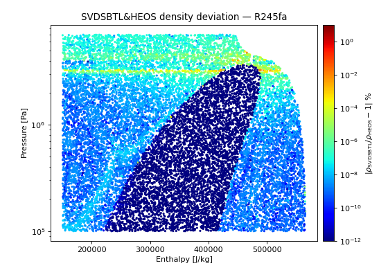
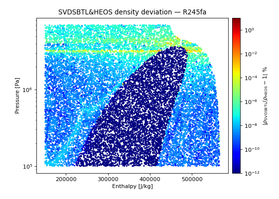
The figure below shows the density deviation of SVDSBTL&HEOS from the underlying HEOS truth source over the full \((h, p)\) envelope of R245fa. Sample density 20,000 random \((h, p)\) points (matching the tabular-interpolation accuracy figure for the BICUBIC / TTSE backends).

(Source code, png, .pdf)

For the IF97-sourced SVDSBTL on water, the per-property fail-map figure in IF97 Conformance and Timing shows the equivalent — same \((h, p)\)-coloured deviation pattern but classified against the IAPWS G13-15 conformance budgets rather than reported as raw relative error.

For the underlying SVD compression math — why a rank-\(r\) SVD of a smooth function on a rectangle gives \(O(r^{-\infty})\) error decay, why the natural cubic spline beats finite-difference slopes for the Hermite per-mode interpolation, and the f(x, y) = \exp(-x^2 - y^2) rank-2 worked example — see Low-rank SVD lookup for 2D property tables.

Programmatic access

Beyond the high-level AbstractState API, the C++ class CoolProp::SVDSBTLBackend exposes:

• fast_evaluate for batched cache-bypassing evaluation — also bound to Python (see the example above).

• registered_input_pairs() for introspection (which surfaces did this instance load). C++-only; not bound to Python.

Runtime overrides to the critical-patch geometry currently require reconstructing the backend with an updated critical_patch.bbox options blob; there is no in-place setter.

All other AbstractState methods (rhomass, hmass, smass, viscosity, conductivity, T_critical, Ttriple, etc.) work identically to other backends.