Robust, fast \(H\),\(S\) flash#

This page describes the algorithm CoolProp uses to solve the enthalpy–entropy flash HmolarSmolar_INPUTS for pure fluids: given molar \((h,s)\), recover the thermodynamic state \((T,\rho)\) (single-phase) or \((T,Q)\) (two-phase).

Historically this was the last input pair without a superancillary-accelerated happy path. The legacy solver seeded a Newton iteration from a random \((T,p)\) guess (HS_flash_generate_TP_singlephase_guess), which is the root cause of the failures reported in issue #2022 and relatives. The current implementation replaces that with a deterministic cascade of homotopy solvers that is 100% robust across the fluid library and roughly 1000× faster on total wall time than the legacy path, while never returning a wrong (metastable) root.

The difficulty#

Single-phase \(H\),\(S\) is a genuine 2-D inversion \((h,s)\mapsto(T,\rho)\) with two obstructions:

The two-phase dome. A straight Newton path from a poor guess can wander into the two-phase region, where there is no single-phase solution.
Apparent non-uniqueness. For some states (notably dense, supercritical hydrogen) two distinct \((T,\rho)\) reproduce the same \((h,s)\) and are both mechanically stable (\(\left.\partial p/\partial\rho\right|_T>0\)). Only one is physical.

Both are resolved below.

Strategy: anchor where a matching-entropy state must exist, then march#

Each leg is a homotopy continuation. The idea: instead of solving a hard problem from a blind guess, start from an easy problem whose answer you already know, then deform it continuously into the hard one, nudging the solution along at each step so you never lose it. Concretely, introduce a parameter that sweeps from 0 to 1: at 0 the problem is trivial (an exactly-known anchor state), at 1 it is the target \((h,s)\). Taking small steps in that parameter and re-converging with a few Newton iterations at each one traces a continuous path from the anchor to the answer – and as long as that path never enters the two-phase dome, every point on it is a valid single-phase state, so the march cannot fall into a non-physical region.

Every leg of the cascade is such a march; they differ only in where the easy anchor lives – each a place where a state of the target entropy is guaranteed to exist:

leg	anchor	owns
saturation anchor	the saturated state whose entropy equals \(s\)	sub-critical liquid/vapor (≈99.9%)
supercritical isentrope	the \(T=T_{\max}\) isotherm at the density matching \(s\)	supercritical targets
ideal-gas departure	the ideal-gas limit (\(\lambda=0\), no dome at all)	universal backstop

The cascade tries them in order and accepts the first result that passes the acceptance gate.

Leg 1 — saturation anchor#

Using the fluid’s superancillaries (Chebyshev fits of the saturation curve, evaluated with no EOS calls), find every saturation temperature \(T_0\) where the saturated entropy equals the target: \(s_{\rm sat}(T_0)=s\). This uses the native \(S\)-inversion get_all_intersections('S', s), which returns all roots and so handles the retrograde (non-monotone) saturated entropy of siloxanes. The anchor is that saturated state, \((T_0,\ \rho_0=\rho_{\rm sat}(T_0))\), on the branch (liquid or vapor) whose entropy matches; ties are broken by enthalpy closeness to the target.

Because the anchor entropy already equals \(s\), the \((h,s)\) chord holds entropy fixed — the path is the isentrope \(s=\text{const}\), and only the enthalpy is driven from the saturated value to the target. When the target entropy lies outside the saturation band (no such saturated state exists), this leg defers to leg 2.

Leg 2 — supercritical isentrope#

For a supercritical target there is no saturated state at its entropy, so we anchor on the dome-free hot isotherm \(T=T_{\max}\) at the density \(\rho_0\) where \(s(T_{\max},\rho_0)=s\) (entropy is monotone in density along an isotherm, so this is a clean 1-D bracketed solve). Marching the isentrope from \(T_{\max}\) downward to a supercritical target stays at \(T>T_c\) the whole way and so never touches the dome — structurally guaranteeing a valid path.

Leg 3 — ideal-gas departure homotopy#

As a universal backstop, scale the residual (real-fluid) Helmholtz energy by a parameter \(\lambda\in[0,1]\):

\[\alpha(\tau,\delta;\lambda) = \alpha^0(\tau,\delta) + \lambda\,\alpha^{\mathrm r}(\tau,\delta).\]

At \(\lambda=0\) the fluid is an ideal gas — it has no two-phase dome, and the \((h,s)\) inversion is two trivial monotone 1-D rootfinds (for \(T\) then \(\rho\)). Continuing \(\lambda:0\to1\) grows the real fluid (and its dome) from nothing while the corrector tracks the stable branch. All properties along the way come from the cached \(\alpha^0\) / \(\alpha^{\mathrm r}\) derivatives, so this leg needs no superancillary.

The corrector: Newton in \((T,\ w=\ln\rho)\)#

Working in \(w=\ln\rho\) makes \(\rho>0\) automatic and conditions the entropy direction. At each homotopy step the corrector solves \(h(T,\rho)=h_\lambda,\ s(T,\rho)=s_\lambda\) by Newton, with the Jacobian columns \(\partial/\partial T\) and \(\partial/\partial w=\rho\,\partial/\partial\rho\). Two guards keep it physical:

Mechanical-stability damping — each step is halved until \(\left.\partial p/\partial\rho\right|_T>0\), keeping the corrector on the stable branch.
Domain clamp with slack — \(T\) is kept in \([\,0.98\,T_{\min},\ 1.5\,T_{\max}]\). The 2% slack below \(T_{\min}\) matters near the triple point: the compressed-liquid isentrope folds a few hundredths of a percent below \(T_{\min}\) (water’s density anomaly) before climbing back to an in-range target, and a hard clamp would stall there.

Failed steps trigger adaptive subdivision (double the number of \(\lambda\) steps).

Acceptance gate and the uniqueness theorem#

A candidate \((T,\rho)\) is accepted only if it

reproduces \((h,s)\) to tolerance,
lies in \([T_{\min},T_{\max}]\),
is fully intrinsically stable: \(\left.\partial p/\partial\rho\right|_T>0\) (mechanical) and \(c_v>0\) (thermal), and
lies outside the two-phase dome.

Conditions 3–4 are what make the answer unique and physical. At fixed entropy, \(\mathrm{d}h = v\,\mathrm{d}p\), and along the adiabat \(\left.\partial p/\partial v\right|_s<0\) for any stable state, so \(h\) is strictly monotone in \(v\) at fixed \(s\): the map \((h,s)\to(T,\rho)\) is injective over the fully stable region. The apparent non-uniqueness (e.g. the dense supercritical-hydrogen pair) is not a real feature — the spurious second root has \(c_v<0\) (thermally unstable, an EOS extrapolation artifact), so the \(c_v>0\) gate removes it. Because the gate certifies the unique physical root, the solver never needs to know the true answer in advance — a matching, stable, outside-dome root is the answer.

For a two-phase \((h,s)\) there is no stable single-phase root: every cascade leg lands on an in-dome metastable state and is rejected by condition 4. The cascade therefore fails cleanly, and the dispatcher falls through to the EOS-exact two-phase solve (the \(Q_h=Q_s\) saturation problem, the \(H\),\(S\) analogue of the \(D\)+\(X\) happy path).

Try it#

The happy path is engaged automatically by PropsSI / the low-level interface for pure fluids when superancillaries are enabled. Below we round-trip a single-phase state and a two-phase state, then time the flash with the low-level interface – a reused AbstractState calling update(HmolarSmolar_INPUTS, ...) – so the measurement reflects the flash cost itself rather than the per-call string-parsing/factory overhead of PropsSI. The superancillary path is toggled with the ENABLE_SUPERANCILLARIES config flag.

[1]:

import time
import CoolProp.CoolProp as CP

fluid = 'Water'
# A single-phase reference state at (p, T); read off its (h, s)
p, T = 50e6, 700.0  # supercritical water
h = CP.PropsSI('Hmolar', 'P', p, 'T', T, fluid)
s = CP.PropsSI('Smolar', 'P', p, 'T', T, fluid)

# Recover (T, rho) from (h, s)
T_rt   = CP.PropsSI('T',      'Hmolar', h, 'Smolar', s, fluid)
rho_rt = CP.PropsSI('Dmolar', 'Hmolar', h, 'Smolar', s, fluid)
rho_ref = CP.PropsSI('Dmolar', 'P', p, 'T', T, fluid)
print(f'single-phase: T {T:.4f} -> {T_rt:.4f} K, rho {rho_ref:.3f} -> {rho_rt:.3f} mol/m^3')

single-phase: T 700.0000 -> 700.0000 K, rho 27256.484 -> 27256.484 mol/m^3

[2]:

# Two-phase round-trip: take a (T, Q) state, read (h, s), recover (T, Q)
Tsat, Q = 450.0, 0.3
h2 = CP.PropsSI('Hmolar', 'T', Tsat, 'Q', Q, fluid)
s2 = CP.PropsSI('Smolar', 'T', Tsat, 'Q', Q, fluid)
T2 = CP.PropsSI('T', 'Hmolar', h2, 'Smolar', s2, fluid)
Q2 = CP.PropsSI('Q', 'Hmolar', h2, 'Smolar', s2, fluid)
print(f'two-phase:    T {Tsat:.4f} -> {T2:.4f} K, Q {Q:.4f} -> {Q2:.4f}')

two-phase:    T 450.0000 -> 450.0000 K, Q 0.3000 -> 0.3000

[3]:

# Low-level timing: reuse one AbstractState and call update() directly, so the
# per-call PropsSI overhead (string parsing, backend lookup) is excluded.
state = CP.AbstractState('HEOS', fluid)
HS = CP.HmolarSmolar_INPUTS
state.update(HS, h, s)  # warm up

def time_hs(n=20000):
    t0 = time.perf_counter()
    for _ in range(n):
        state.update(HS, h, s)
    return 1e6 * (time.perf_counter() - t0) / n  # us per flash

CP.set_config_bool(CP.ENABLE_SUPERANCILLARIES, True)
us_fast = time_hs()
CP.set_config_bool(CP.ENABLE_SUPERANCILLARIES, False)
us_legacy = time_hs()
CP.set_config_bool(CP.ENABLE_SUPERANCILLARIES, True)  # restore
print(f'happy path: {us_fast:6.1f} us/flash   legacy: {us_legacy:8.1f} us/flash   speedup: {us_legacy/us_fast:5.1f}x')

happy path:   91.3 us/flash   legacy:   2823.0 us/flash   speedup:  30.9x

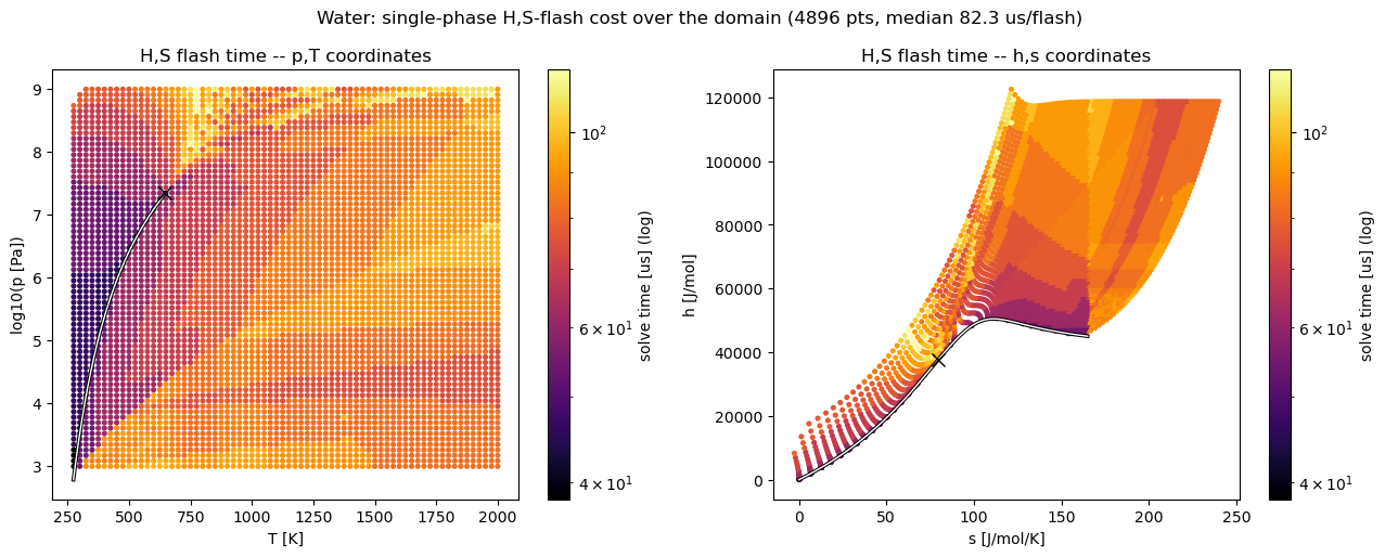
Performance map#

The figure below is produced live by the next code cell: it sweeps a dense single-phase \((\log p, T)\) grid over water’s domain, times the \(H\),\(S\) flash at each point through the low-level interface, and plots the solve time in both \(p\)–\(T\) and \(h\)–\(s\) coordinates (saturation curve / two-phase dome overlaid). The cascade solves the body of the domain with the saturation-anchor leg and a thin band just above the critical point with the supercritical-isentrope leg; across the whole domain it is uniformly cheap — tens of microseconds per flash, with no heavy tail — which is what the time map below shows.

A richer map — EOS-evaluation count and which cascade leg solved each point, in addition to time — comes from the C++ [HS_watermap] test together with CoolProp.Plots.HSFlashTimingMap. The eval-count and per-leg attribution live in the test harness, not the public Python API, so they cannot be regenerated in this notebook; the live figure below therefore shows solve time only. Across 130 pure fluids and ~190k single-phase points the full map shows the cascade solving 100% with 0 regressions against the legacy path, at a mean of ~16 EOS evaluations and a worst case under 40 (vs the legacy heavy tail of ~0.5 s on the hardest near-critical points). To reproduce it:

./build_rel/CatchTestRunner "[HS_watermap]"          # writes water_hs_map.csv
python -m CoolProp.Plots.HSFlashTimingMap water_hs_map.csv   # --coords {pt,hs,both}

[4]:

import time
import numpy as np
import matplotlib.pyplot as plt
from matplotlib.colors import LogNorm
import CoolProp.CoolProp as CP

fluid = 'Water'
ref   = CP.AbstractState('HEOS', fluid)   # source of (h, s) at each (p, T)
state = CP.AbstractState('HEOS', fluid)   # the timed H,S flash
HS = CP.HmolarSmolar_INPUTS
CP.set_config_bool(CP.ENABLE_SUPERANCILLARIES, True)

# Phase boundary for the overlay, computed directly from CoolProp: the p,T
# saturation curve, and the closed h,s two-phase dome (up the liquid branch,
# back down the vapor branch), plus the critical point in each coordinate set.
Tt, Tc = CP.PropsSI('Ttriple', fluid), CP.PropsSI('Tcrit', fluid)
Tsat = np.linspace(Tt, Tc, 240)
psat = CP.PropsSI('P', 'T', Tsat, 'Q', 0, fluid)
hL = CP.PropsSI('Hmolar', 'T', Tsat, 'Q', 0, fluid); sL = CP.PropsSI('Smolar', 'T', Tsat, 'Q', 0, fluid)
hV = CP.PropsSI('Hmolar', 'T', Tsat, 'Q', 1, fluid); sV = CP.PropsSI('Smolar', 'T', Tsat, 'Q', 1, fluid)
dome_s = np.concatenate([sL, sV[::-1]]); dome_h = np.concatenate([hL, hV[::-1]])
crit_pt = (Tc, np.log10(psat[-1]))
crit_hs = (0.5 * (sL[-1] + sV[-1]), 0.5 * (hL[-1] + hV[-1]))

# Single-phase (log p, T) sweep over water's domain.  Every (p, T) pair is a
# single-phase state (the saturation line is measure-zero), so we read (h, s)
# off a P,T flash and then time the H,S inversion that has to recover it.
Tmin = CP.PropsSI('Tmin', fluid) + 1.0
Tmax = CP.PropsSI('Tmax', fluid)
pmin, pmax = 1e3, CP.PropsSI('pmax', fluid)
NT, NP, REPS = 70, 70, 5                   # grid resolution and per-point timing repeats

Tgrid   = np.linspace(Tmin, Tmax, NT)
log10ps = np.linspace(np.log10(pmin), np.log10(pmax), NP)

Tg, hg, sg, lpg, usg = [], [], [], [], []
n_skip, skip_reasons = 0, {}                # keep the sweep resilient but the failures visible
for log10p in log10ps:
    p = 10.0 ** log10p
    for T in Tgrid:
        try:
            ref.update(CP.PT_INPUTS, p, float(T))
            h, s = ref.hmolar(), ref.smolar()
            best = np.inf
            for _ in range(REPS):          # min over repeats rejects scheduler noise
                t0 = time.perf_counter()
                state.update(HS, h, s)
                best = min(best, time.perf_counter() - t0)
        except Exception as err:           # a flash that rejects the point: skip it, but count + report it
            n_skip += 1
            skip_reasons[type(err).__name__] = skip_reasons.get(type(err).__name__, 0) + 1
            continue
        Tg.append(float(T)); hg.append(h); sg.append(s)
        lpg.append(log10p); usg.append(best * 1e6)

Tg, hg, sg, lpg, usg = map(np.array, (Tg, hg, sg, lpg, usg))
print('{0} single-phase points timed, {1} skipped; median {2:.1f} us, p95 {3:.1f} us, max {4:.1f} us'.format(
    len(usg), n_skip, np.median(usg), np.percentile(usg, 95), usg.max()))
if skip_reasons:
    print('  skipped-point exceptions:', ', '.join('{0}x{1}'.format(v, k) for k, v in sorted(skip_reasons.items())))

norm = LogNorm(vmin=max(usg.min(), 1e-2), vmax=usg.max())
fig, (axpt, axhs) = plt.subplots(1, 2, figsize=(13, 5.2))

for ax, x, y, xl, yl, bx, by, cp, ttl in (
        (axpt, Tg, lpg, 'T [K]', 'log10(p [Pa])', Tsat, np.log10(psat), crit_pt, 'p,T coordinates'),
        (axhs, sg, hg, 's [J/mol/K]', 'h [J/mol]', dome_s, dome_h, crit_hs, 'h,s coordinates')):
    sc = ax.scatter(x, y, c=usg, s=7, cmap='inferno', norm=norm)
    ax.set(xlabel=xl, ylabel=yl, title='H,S flash time -- ' + ttl)
    fig.colorbar(sc, ax=ax, label='solve time [us] (log)')
    ax.plot(bx, by, 'k-', lw=2.5); ax.plot(bx, by, 'w-', lw=1.0)   # saturation curve / dome
    ax.plot(*cp, 'x', color='w', mec='k', ms=9)                    # critical point

fig.suptitle('{0}: single-phase H,S-flash cost over the domain ({1} pts, median {2:.1f} us/flash)'.format(
    fluid, len(usg), np.median(usg)))
fig.tight_layout()

4896 single-phase points timed, 4 skipped; median 82.3 us, p95 93.8 us, max 117.8 us
  skipped-point exceptions: 4xValueError

References & implementation#

Implementation: FlashRoutines::HS_flash in src/Backends/Helmholtz/FlashRoutines.cpp (the hs_corrector / hs_leg_* / hs_cascade helpers), mirroring the HSU_D_flash hybrid.
Characterization & stress tests: src/Tests/CoolProp-Tests-HS.cpp ([HS_grid], [HS_casc], [HS_stress], [HS_prod2ph]).
Superancillaries: see the Superancillaries page.
Original issue: #2022.

Table of Contents