Cubic Equations of State #

Introduction #

CoolProp (as of version 6) comes with two standard cubic equations of state: Soave-Redlich-Kwong (SRK) and Peng-Robinson (PR). These two equations of state can be expressed in a common, generalized form:

\[p = \frac{RT}{v-b} + \frac{a}{(v+\Delta_1b)(v+\Delta_2b)}\]

where for pure fluids, \(a\) and \(b\) are not composition dependent, whereas for mixtures, they have composition dependence. These cubic EOS can be converted to a form that is compatible with the multi-fluid model used in CoolProp according to the analysis in Bell and Jager [204].

The motivations for the use of cubic EOS are twofold:

The only required information for the EOS are \(T_c\), \(p_c\), and the acentric factor of the pure fluids
They are much more computationally efficient (see below)

Caveats#

Warning

NOT ALL PROPERTIES ARE AVAILABLE AS INPUTS/OUTPUTS

Only a limited subset of properties are available currently. You can do:

Flash calculations with TP, PQ, DT, QT inputs
Calculation of mixture critical point(s)
Calculation of some mixture flashes

Pure Fluids #

Usage#

As a user, in the high-level interface, all that you have to do to evaluate properties using the SRK or PR backends is to change the backend name.

In [1]: import CoolProp.CoolProp as CP

# The multi-parameter Helmholtz backend
In [2]: CP.PropsSI("T","P",101325,"Q",0,"HEOS::Propane")
Out[2]: 231.03621464432234

# SRK
In [3]: CP.PropsSI("T","P",101325,"Q",0,"SRK::Propane")
Out[3]: 231.2732911779881

# Peng-Robinson
In [4]: CP.PropsSI("T","P",101325,"Q",0,"PR::Propane")
Out[4]: 230.9620404030514

The same holds for the low-level interface:

In [5]: import CoolProp.CoolProp as CP

In [6]: AS = CP.AbstractState("SRK", "Propane"); AS.update(CP.QT_INPUTS, 0, 300); print(AS.p())
1008665.2337895618

In [7]: AS = CP.AbstractState("PR", "Propane"); AS.update(CP.QT_INPUTS, 0, 300); print(AS.p())
997429.8169997159

All the fluids available in CoolProp are also available through the cubic equations of state. The fluids can be extended according to the analysis shown below

Speed#

The increase in speed for evaluating properties from a cubic EOS is one of the primary motivations. Here we show an example of the speedup to VLE calculations:

In [8]: import CoolProp.CoolProp as CP

# The multi-parameter Helmholtz backend
In [9]: AS = CP.AbstractState("HEOS", "Propane")

In [10]: %timeit AS.update(CP.QT_INPUTS, 0, 300)
446 ns +- 0.51 ns per loop (mean +- std. dev. of 7 runs, 1,000,000 loops each)

# The cubic SRK backend
In [11]: AS = CP.AbstractState("SRK", "Propane")

In [12]: %timeit AS.update(CP.QT_INPUTS, 0, 300)
2.12 us +- 2.08 ns per loop (mean +- std. dev. of 7 runs, 100,000 loops each)

And here, we run the PT flash

In [13]: import CoolProp.CoolProp as CP

# The multi-parameter Helmholtz backend
In [14]: AS = CP.AbstractState("HEOS", "Propane")

In [15]: AS.specify_phase(CP.iphase_gas)

In [16]: %timeit AS.update(CP.PT_INPUTS, 101325, 300)
4.43 us +- 2.74 ns per loop (mean +- std. dev. of 7 runs, 100,000 loops each)

# The cubic SRK backend
In [17]: AS = CP.AbstractState("SRK", "Propane")

In [18]: AS.specify_phase(CP.iphase_gas)

In [19]: %timeit AS.update(CP.PT_INPUTS, 101325, 300)
312 ns +- 0.0796 ns per loop (mean +- std. dev. of 7 runs, 1,000,000 loops each)

As you can see, the speed difference is quite significant

Superancillaries for SRK and PR#

For an additional speedup on saturation calculations, piecewise Chebyshev superancillary expansions (Bell and Deiters [205], ported from teqp) are available for pure fluids with the SRK and PR backends. They return \(p^{\mathrm{sat}}(T)\), \(\rho'(T)\), and \(\rho''(T)\) directly from closed-form polynomials — no iterative flash — at an accuracy better than 10^-3 relative to the cubic EOS result over the full saturation dome up to \(T_c\).

Two entry points are provided on the AbstractState (low-level interface only):

update_QT_pure_superanc(Q, T) — populates the full two-phase state (same fields as update(QT_INPUTS, Q, T)) using the superancillary instead of a full VLE flash.
saturation_ancillary(param, Q, iT, T) — returns a single saturation property (iP or iDmolar) without updating state.

Warning

Superancillaries are only available for pure fluids with the SRK and PR backends, and only with T as the independent variable (T must satisfy \(T \le T_c\)). They are not used transparently by PropsSI — you must use the low-level interface explicitly.

In [20]: import CoolProp.CoolProp as CP

In [21]: AS = CP.AbstractState("PR", "Propane")

# Full VLE flash through the cubic EOS
In [22]: %timeit AS.update(CP.QT_INPUTS, 1, 300)
1.73 us +- 0.454 ns per loop (mean +- std. dev. of 7 runs, 1,000,000 loops each)

# Same state populated from the superancillary
In [23]: %timeit AS.update_QT_pure_superanc(1, 300)
532 ns +- 1.04 ns per loop (mean +- std. dev. of 7 runs, 1,000,000 loops each)

# Single saturation property (no state update)
In [24]: %timeit AS.saturation_ancillary(CP.iP, 0, CP.iT, 300)
255 ns +- 0.721 ns per loop (mean +- std. dev. of 7 runs, 1,000,000 loops each)

On a typical modern laptop this corresponds to roughly a 5–6x speedup for update_QT_pure_superanc relative to the full cubic flash, and roughly 9–10x for saturation_ancillary on a single property; exact numbers are hardware-dependent.

Mixtures #

Interaction Parameters#

For mixtures, cubic EOS (and their modifications) are heavily used. Cubic EOS allow for reasonable prediction of VLE with only one adjustable parameter, at least for reasonable mixtures. CoolProp does not come with any values for the \(k_{ij}\) parameter, but it is straightforward to add it yourself.

Warning

The ability to adjust interaction parameters is ONLY available in the low-level interface

Warning

When you call set_binary_interaction_double, it only applies to the given instance of the AbstractState

In [25]: import CoolProp.CoolProp as CP

In [26]: AS = CP.AbstractState("SRK", "Methane&Ethane")

In [27]: AS.set_mole_fractions([0.5, 0.5])

In [28]: AS.update(CP.QT_INPUTS, 0, 120); print(AS.p())
104455.58354040685

In [29]: AS.set_binary_interaction_double(0,1,"kij",-0.05)

In [30]: AS.update(CP.QT_INPUTS, 0, 120); print(AS.p())
82024.35148483743

Critical Points#

According to a forthcoming paper from Bell et al., it is possible to calculate critical points of mixtures from cubic EOS. For instance, here is how to calculate all the critical points (there can be more than one) that are found for an equimolar mixture of methane and ethane:

In [31]: import CoolProp.CoolProp as CP

In [32]: AS = CP.AbstractState("SRK", "Methane&Ethane")

In [33]: AS.set_mole_fractions([0.5, 0.5])

In [34]: pts = AS.all_critical_points()

In [35]: [(pt.T, pt.p, pt.rhomolar, pt.stable) for pt in pts]
Out[35]: [(266.3228193395559, 6859367.557158955, 7895.097555224677, True)]

Cubics in multi-fluid model#

The cubic equations of state can also be used to replace a single fluid in a multi-fluid model (the GERG-like model) (see Bell and Jager [204]), by appending either -SRK or -PengRobinson to the fluid name. For instance, you could calculate the NBP with both the conventional multi-fluid model (as in GERG), or translating both to cubic equations of state

In [36]: import CoolProp.CoolProp as CP

# With the normal multi-fluid model
In [37]: CP.PropsSI('T', 'P', 101325, 'Q', 0, 'HEOS::Methane-SRK[0.4]&Ethane-SRK[0.6]')
Out[37]: 122.0132797624242

# With both fluids using cubic translations in the multi-fluid model
In [38]: CP.PropsSI('T', 'P', 101325, 'Q', 0, 'HEOS::Methane[0.4]&Ethane[0.6]')
Out[38]: 121.5191036195154

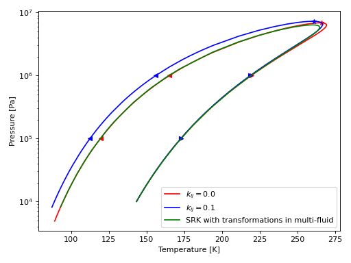
Detailed Example#

Here we plot phase envelopes and critical points for an equimolar methane/ethane mixture

(Source code, png, .pdf)

Adding your own fluids #

The cubic fluids in CoolProp are defined based on a JSON format, which could yield something like this for a FAKE (illustrative) fluid. For instance if we had the file fake_fluid.json (download it here: fake_fluid.json):

[
  {
    "CAS": "000-0-00", 
    "Tc": 400.0, 
    "Tc_units": "K", 
    "acentric": 0.1, 
    "aliases": [
    ], 
    "molemass": 0.04, 
    "molemass_units": "kg/mol", 
    "name": "FAKEFLUID", 
    "pc": 4000000.0, 
    "pc_units": "Pa"
  }
]

The JSON-formatted fluid information is validated against the JSON schema, which can be obtained by calling the get_global_param_string function:

In [39]: import CoolProp.CoolProp as CP

# Just the first bit of the schema (it's a bit large; see below for the complete schema)
In [40]: CP.get_global_param_string("cubic_fluids_schema")[0:60]
Out[40]: '{\n  "$schema": "http://json-schema.org/draft-04/schema#",\n  '

A JSON schema defines the structure of the data, and places limits on the values, defines what values must be provided, etc.. There are a number of online tools that can be used to experiment with and validate JSON schemas: http://www.jsonschemavalidator.net , http://jsonschemalint.com/draft4/.

In [41]: import CoolProp.CoolProp as CP, json

# Normally you would read it from a file!
In [42]: fake_fluids = [
   ....:                   {
   ....:                     "CAS": "000-0-00",
   ....:                     "Tc": 400.0,
   ....:                     "Tc_units": "K",
   ....:                     "acentric": 0.1,
   ....:                     "aliases": [
   ....:                     ],
   ....:                     "molemass": 0.04,
   ....:                     "molemass_units": "kg/mol",
   ....:                     "name": "FAKEFLUID",
   ....:                     "pc": 4000000.0,
   ....:                     "pc_units": "Pa"
   ....:                   }
   ....:               ]
   ....: 

# Adds fake fluid for both SRK and PR backends since they need the same parameters from the same internal library
In [43]: CP.add_fluids_as_JSON("PR", json.dumps(fake_fluids))

In [44]: CP.PropsSI("T","P",101325,"Q",0,"SRK::FAKEFLUID")
Out[44]: 247.09825205570266

# Put in a placeholder interaction parameter (all beta and gamma values are 1.0)
In [45]: CP.apply_simple_mixing_rule("000-0-00", CP.get_fluid_param_string("Ethane","CAS"), "Lorentz-Berthelot")

# Once a fluid has been added to the cubic library, it can be used in the multi-fluid model
In [46]: CP.PropsSI("T","P",101325,"Q",0,"HEOS::FAKEFLUID-SRK[0.3]&Ethane-SRK[0.7]")
Out[46]: 190.9405276513907

Complete fluid schema#

For completeness, here is the whole JSON schema used for the cubic backends:

In [47]: import CoolProp.CoolProp as CP

In [48]: print(CP.get_global_param_string("cubic_fluids_schema"))
{
  "$schema": "http://json-schema.org/draft-04/schema#",
  "title": "Fluid for cubic EOS in CoolProp",
  "items": {
    "properties": {
      "name": {
        "description": "Name of the fluid",
        "type": "string"
      },
      "CAS": {
        "description": "CAS registry number of the fluid",
        "type": "string"
      },
      "Tc": {
        "description": "Critical temperature (K)",
        "type": "number",
        "minimum": 0.1,
        "maximum": 20000
      },
      "pc": {
        "description": "Critical pressure (Pa)",
        "type": "number",
        "minimum": 0,
        "maximum": 500000000
      },
      "rhomolarc": {
        "description": "Critical density (mol/m^3)",
        "type": "number",
        "minimum": 0.1,
        "maximum": 2000000
      },
      "rhomolarc_units": {
        "description": "Units of the critical density provided",
        "enum": [
          "mol/m^3",
          "kg/m^3"
        ]
      },
      "acentric": {
        "description": "Acentric factor (-)",
        "type": "number",
        "minimum": -10,
        "maximum": 10
      },
      "molemass": {
        "description": "Molar mass (kg/mol)",
        "type": "number",
        "minimum": 0,
        "maximum": 1
      },
      "molemass_units": {
        "description": "Units of the molar mass provided",
        "enum": [
          "kg/mol"
        ]
      },
      "pc_units": {
        "description": "Units of the critical pressure",
        "enum": [
          "Pa"
        ]
      },
      "Tc_units": {
        "description": "Units of the critical temperature",
        "enum": [
          "K"
        ]
      },
      "aliases": {
        "type": "array",
        "items": {
          "type": "string"
        },
        "minItems": 0
      },
      "alpha": {
        "description": "The alpha function being used",
        "properties": {
          "type":{
            "enum": [
              "Twu",
              "Mathias-Copeman",
              "default"
            ]
          },
          "c":{
              "type": "array",
              "items": {
                "type": "number"
              },
              "minItems": 3,
              "maxItems": 3
          }
        }
      }
    },
    "required": [
      "name",
      "CAS",
      "Tc",
      "Tc_units",
      "pc",
      "pc_units",
      "acentric",
      "molemass",
      "molemass_units"
    ]
  },
  "type": "array"
}

Table of Contents

Cubic Equations of State #

Introduction #

Caveats#

Pure Fluids #

Usage#

Speed#

Superancillaries for SRK and PR#

Mixtures #

Interaction Parameters#

Critical Points#

Cubics in multi-fluid model#

Detailed Example#

Adding your own fluids #

Complete fluid schema#

This Page

Table of Contents

Cubic Equations of State#

Introduction#

Caveats#

Pure Fluids#

Usage#

Speed#

Superancillaries for SRK and PR#

Mixtures#

Interaction Parameters#

Critical Points#

Cubics in multi-fluid model#

Detailed Example#

Adding your own fluids#

Complete fluid schema#

This Page

Cubic Equations of State #

Introduction #

Pure Fluids #

Mixtures #

Adding your own fluids #