R124#
References#
Equation of State#
B. de Vries, R. Tillner-Roth, and H.D. Baehr. Thermodynamic Properties of HCFC 124. In 19th International Congress of Refrigeration, The Hague, The Netherlands, 582–589. 1995.Thermal Conductivity#
Marcia L. Huber, Arno Laesecke, and Richard A. Perkins. Model for the Viscosity and Thermal Conductivity of Refrigerants, Including a New Correlation for the Viscosity of R134a. Ind. Eng. Chem. Res., 42:3163–3178, 2003. doi:10.1021/ie0300880.Viscosity#
Ian H. Bell and Arno Laesecke. Viscosity of refrigerants and other working fluids from residual entropy scaling . In 16th International Refrigeration and Air Conditioning Conference at Purdue, July 11-14, 2016. 2016.Surface Tension#
A. Mulero, I. Cachadiña, and M. I. Parra. Recommended Correlations for the Surface Tension of Common Fluids. J. Phys. Chem. Ref. Data, 41(4):043105–1:13, 2012. doi:10.1063/1.4768782.Molecular Structure#
R124 — 3D conformer (interactive: click and drag to rotate)
Fluid Information#
Parameter, Value |
|
|---|---|
General |
|
Molar mass [kg/mol] |
0.1364762 |
CAS number |
2837-89-0 |
ASHRAE class |
A1 |
Formula |
C2ClF4H |
Acentric factor |
0.2880950842214292 |
InChI |
InChI=1S/C2HClF4/c3-1(4)2(5,6)7/h1H |
InChIKey |
BOUGCJDAQLKBQH-UHFFFAOYSA-N |
SMILES |
C(C(F)(F)F)(F)Cl |
ChemSpider ID |
16841 |
Limits |
|
Maximum temperature [K] |
470.0 |
Maximum pressure [Pa] |
40000000.0 |
Triple point |
|
Triple point temperature [K] |
120.0 |
Triple point pressure [Pa] |
0.026738623617928323 |
Critical point |
|
Critical point temperature [K] |
395.4279607732047 |
Critical point density [kg/m3] |
559.293168797007 |
Critical point density [mol/m3] |
4098.100392573994 |
Critical point pressure [Pa] |
3624482.5109438105 |
Reducing point |
|
Reducing point temperature [K] |
395.425 |
Reducing point density [mol/m3] |
4103.279546177282 |
REFPROP Validation Data#
Note
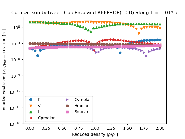
This figure compares the results generated from CoolProp and those generated from REFPROP. They are all results obtained in the form \(Y(T,\rho)\), where \(Y\) is the parameter of interest and which for all EOS is a direct evaluation of the EOS
You can download the script that generated the following figure here: (link to script), right-click the link and then save as… or the equivalent in your browser. You can also download this figure as a PDF.
Consistency Plots#
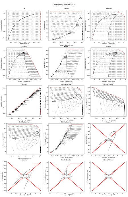
The following figure shows all the flash routines that are available for this fluid. A red + is a failure of the flash routine, a black dot is a success. Hopefully you will only see black dots. The red curve is the maximum temperature curve, and the blue curve is the melting line if one is available for the fluid.
In this figure, we start off with a state point given by T,P and then we calculate each of the other possible output pairs in turn, and then try to re-calculate T,P from the new input pair. If we don’t arrive back at the original T,P values, there is a problem in the flash routine in CoolProp. For more information on how these figures were generated, see CoolProp.Plots.ConsistencyPlots
Note
You can download the script that generated the following figure here: (link to script), right-click the link and then save as… or the equivalent in your browser. You can also download this figure as a PDF.
Flash consistency (HEOS): 18 inconsistent, 0 exceptions, 0 bad-phase across 3 input pair(s).
Download full failure list (CSV)
Failing state points (sample, up to 20 per pair/class)
Pair |
Class |
Region |
P [Pa] |
T [K] |
In1 |
Val1 |
In2 |
Val2 |
Error |
|---|---|---|---|---|---|---|---|---|---|
DmolarP |
INCONSISTENT |
1phase |
10.4241 |
130.046 |
Dmolar |
13382.7 |
P |
10.4241 |
|
DmolarP |
INCONSISTENT |
1phase |
17.9136 |
130.046 |
Dmolar |
13382.7 |
P |
17.9136 |
|
DmolarP |
INCONSISTENT |
1phase |
0.0464092 |
121.1 |
Dmolar |
13554.4 |
P |
0.0464092 |
|
DmolarP |
INCONSISTENT |
1phase |
0.0797531 |
121.1 |
Dmolar |
13554.4 |
P |
0.0797531 |
|
DmolarP |
INCONSISTENT |
1phase |
2.05404 |
138.992 |
Dmolar |
13212 |
P |
2.05404 |
|
DmolarP |
INCONSISTENT |
1phase |
0.235524 |
121.1 |
Dmolar |
13554.4 |
P |
0.235524 |
|
DmolarP |
INCONSISTENT |
1phase |
0.404742 |
121.1 |
Dmolar |
13554.4 |
P |
0.404742 |
|
DmolarP |
INCONSISTENT |
1phase |
0.69554 |
121.1 |
Dmolar |
13554.4 |
P |
0.69554 |
|
DmolarP |
INCONSISTENT |
1phase |
0.69554 |
130.046 |
Dmolar |
13382.7 |
P |
0.69554 |
|
DmolarP |
INCONSISTENT |
1phase |
0.137054 |
121.1 |
Dmolar |
13554.4 |
P |
0.137054 |
|
DmolarP |
INCONSISTENT |
1phase |
0.404742 |
130.046 |
Dmolar |
13382.7 |
P |
0.404742 |
|
DmolarP |
INCONSISTENT |
1phase |
1.19527 |
130.046 |
Dmolar |
13382.7 |
P |
1.19527 |
|
HmolarSmolar |
INCONSISTENT |
2phase |
0.0345634 |
121 |
Hmolar |
6828.4 |
Smolar |
28.1576 |
|
SmolarT |
INCONSISTENT |
1phase |
0.69554 |
121.1 |
Smolar |
28.2622 |
T |
121.1 |
|
SmolarT |
INCONSISTENT |
1phase |
0.404742 |
121.1 |
Smolar |
28.2622 |
T |
121.1 |
|
SmolarT |
INCONSISTENT |
1phase |
0.235524 |
121.1 |
Smolar |
28.2622 |
T |
121.1 |
|
SmolarT |
INCONSISTENT |
1phase |
0.137054 |
121.1 |
Smolar |
28.2622 |
T |
121.1 |
|
SmolarT |
INCONSISTENT |
1phase |
0.0797531 |
121.1 |
Smolar |
28.2622 |
T |
121.1 |
Superancillary Plots#
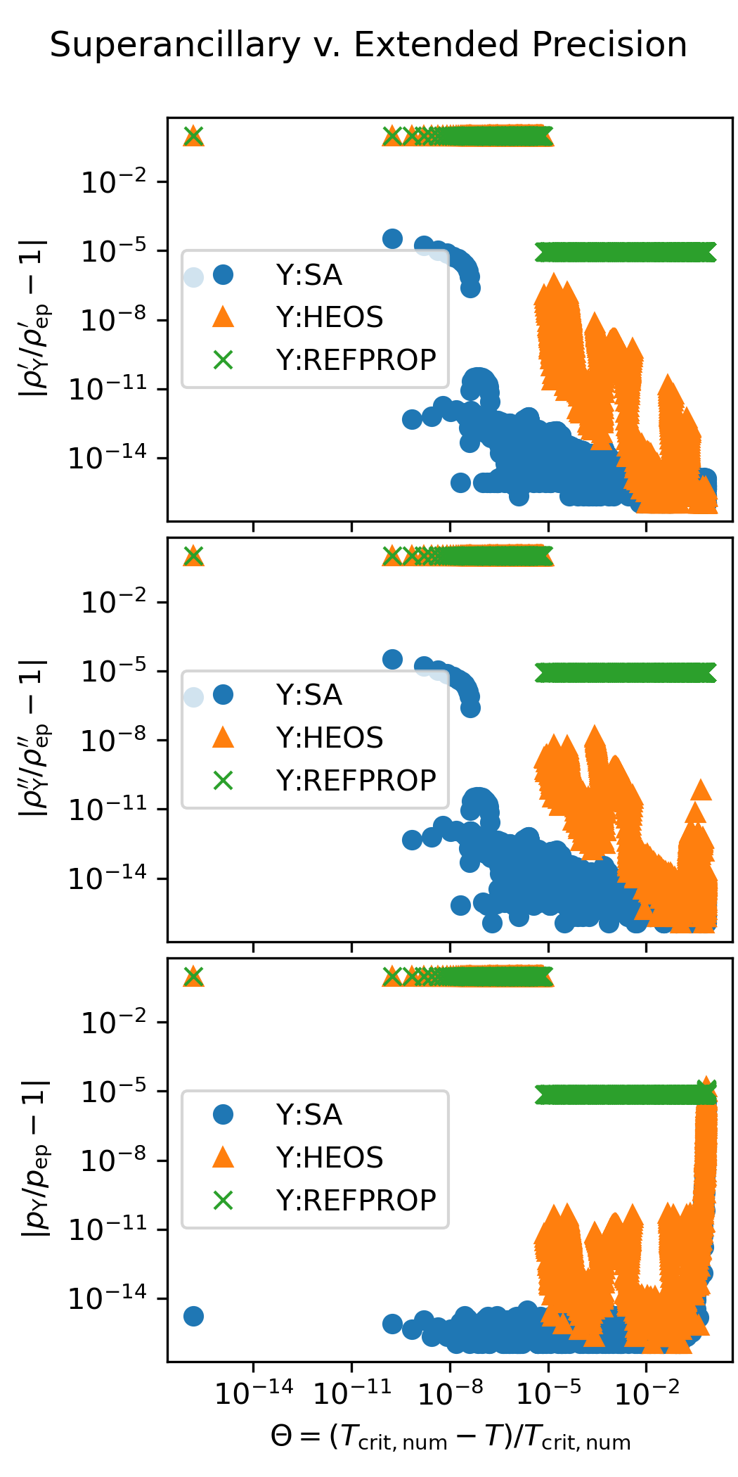
The following figure shows the accuracy of the superancillary functions relative to extended precision calculations carried out in C++ with the teqp library. The results of the iterative calculations with REFPROP and CoolProp are also shown.
Note
You can download the script that generated the following figure here: (link to script), right-click the link and then save as… or the equivalent in your browser. You can also download this figure as a PDF.